Using VLOOKUP function with IF function

Last time we were discussing about complex or nested if function by which we calculated the grades of students. now we can useVLOOKUP function in place of nested if with the grades.

Just use like this
=IF(logical_test,"TRUE",VLOOKUP(lookupvalue,table_array,column_index_no,range_lookup))
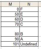by this you can reduce complexity of the previous function we used last time
this time we can use a table like (M1:N7) here with the reference of the grades.
and the function will be like the following

=IF(OR(AND(B2<50,COUNT(B2)=1),AND(C2<50,COUNT(C2)=1),AND(D2<50,COUNT(D2)=1)),"F",VLOOKUP(E2,M1:N7,2,TRUE))

using IF function in excel

The IF function in Excel take three parameters. here is the general form of the function.
=IF(logical_test, value_if_true, value_if_false)
Now we are going to take an example to solve the function along with other functions if necessary

Here we have taken some students marks and you can see their average. If I want to specify the students who passed or who failed by considering their average we can set if function like this